Create a Quarto course from scratch#
In this section we describe how we created an
online course entirely with Quarto.
The main idea was to create a website with all the necessary content to give a brief
introduction to a topic, with a set of slides created with the same content, a
printable version as a pdf, video recordings for each section, all with Python
interactive examples.
Overall structure of the course#
The idea is to create a self-contained course with multiple publishing options
that adapt to the device capabilities. The most comprehensive format to
access the course is in its website format
which includes textual narrative, tables, figures, equations, interactive code and video recordings.
The other format that includes the full narrative, but without interactive code or video, is the printable PDF.
Finally, the reveal.js slides focus on the key points but include the
tables, figures, equations and the interactive code.
In order to generate multiple types of outputs with Quarto it is necessary to
configure the different formats in the _quarto.yml file (See lines 52-84) and
in the quarto markdown file of the specific section (See lines 20-38 of odm.qmd).
The following is a small extract of the configuration in YAML format.
format:
  html:
    theme:
      light: [yeti, mooctai.scss]
      dark: [superhero, mooctai_dark.scss]
    code-link: true
    css: style.css
    toc: true
    number-chapters: true
  reveal.js:
    logo: "../images/logos/tailor_and_uob.svg"
    output-file: slides-intro-to-opt-dec-mak.html
    slide-number: true
    incremental: true
    smaller: false
    auto-stretch: false
    chalkboard: true
  pdf:
    include-in-header:
      - file: packages.tex
      - operators.tex
      - colors.tex
      - definitions.tex
Course narrative and key points#
The course follows a textual narrative explaining the details, but the slides need to concentrate on the main points, leaving out some details. This can be achieved as follows:
::: {.content-hidden when-format="reveal.js"}

Text shown in all formats excepts reveal.js slides.

:::
In order to keep some content in the slides we decided to create lists with the
key points, which can be shown in all formats. We have added a Key Points
title as a subsection in the other formats (an example can be found at
https://tailor-uob.github.io/training-material/cha_odm/odm.html#key-points).
Figures, tables and equations#
Figures, tables and equations can be visualised in all formats and are automatically adjusted to fit the available space of the output format.
Figures can be easily added in plain markdown

which would be rendered as follows:

However, Quarto markdown also allows changes to the style of the image, for
example the alignment and size
{fig-align="center" width="100px"}
or with HTML code as follows.
<img src="images/example.png" alt="Rectangle with the text: example of an
image." style="width=100px">
Warning
Using html syntax to render images in Jupyter Book is not recomended, and
requires the activation of the html_image extension (which is not active in
this roadmap).
Tables can be written in markdown
|  | A  | B  |
|--|----|----|
|1 | A1 | B1 |
|2 | A2 | B2 |
which is rendered as
A |
B |
|
|---|---|---|
1 |
A1 |
B1 |
2 |
A2 |
B2 |
Finally, equations can be written in LaTeX and are interpreted by MathJax.
Equations can be written inline with $E=mc^2$ shown as \(E=mc^2\), or in
display mode:
$$
\begin{equation}
  \mathbb{E}_{j \sim P(\cdot|\vec{x})} (c_{i|j}) = \sum_{j = 1}^K P(C_j|\vec{x}) c_{i|j}.
\end{equation}
$$
which is rendered as
Programming examples#
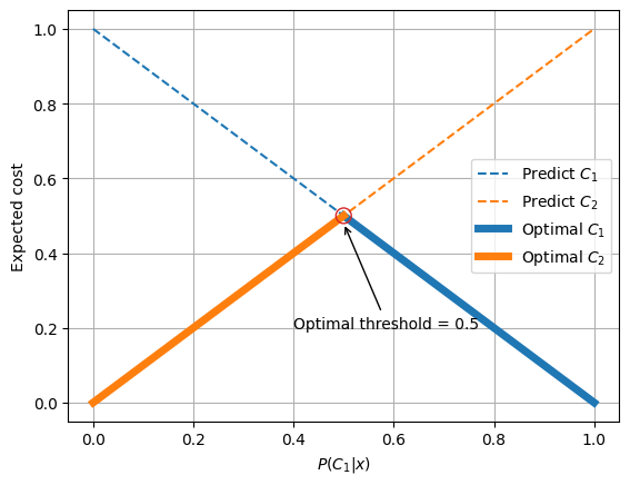
This course is designed for a technical audience that may benefit from programming examples that serve both to teach a concept and learn how to code the example. In this use-case we generate figures based on the explained mathematical concepts. Accessing the source code can provide further intuition to better understand the resulting figures. The next example has been extracted from the use-case which shows the source code and the generated figure below.
import matplotlib.pyplot as plt

C = [[0, 1], [1, 0]]
threshold = (C[0][1] - C[1][1])/(C[0][1] - C[1][1] + C[1][0] - C[0][0])
cost_t = threshold*C[0][0] + (1-threshold)*C[0][1]
plt.grid(True)
plt.plot([0, 1], [C[0][1], C[0][0]], '--', label="Predict $C_1$")
plt.plot([0, 1], [C[1][1], C[1][0]], '--', label="Predict $C_2$")
plt.plot([threshold, 1], [cost_t, C[0][0]], lw=5, color='tab:blue', label="Optimal $C_1$")
plt.plot([0, threshold], [C[1][1], cost_t], lw=5, color='tab:orange', label="Optimal $C_2$")
plt.xlabel('$P(C_1|x)$')
plt.ylabel('Expected cost')
plt.legend()
plt.annotate("Optimal threshold = 0.5", (0.5, 0.48), xytext=(0.4, 0.2),
             arrowprops=dict(arrowstyle='->', facecolor='black'))
plt.scatter(0.5, 0.5, s=100, facecolors='none', edgecolors='tab:red', zorder=10)
plt.show()

Interactive examples#
An important part of the attraction of novel publishing tools is the possibility of creating
interactive and dynamic applications online.
Shinylive is a method that combines Shiny and WebAssembly to
run Python code in your own client web browser. Quarto has a great
integration with this technology, allowing to include code directly in the
markdown that is executed in real time when the page is loaded. The following
code is an example extracted from the use case.
(In this instance we chose not to show the code in the course to focus the learner on the interactive example.)
```{shinylive-python}
#| standalone: true
#| components: viewer
#| viewerHeight: 480

import matplotlib.pyplot as plt
from shiny import App, render, ui
import pandas as pd

app_ui = ui.page_fluid(
    ui.layout_sidebar(
        ui.sidebar(
    ui.input_slider("TP", "Cost True C1",  value=-5, min=-10, max=0),
    ui.input_slider("TN", "Cost True C2",  value=-1, min=-10, max=0),
    ui.input_slider("FN", "Cost False C2", value=10, min=1,   max=10),
    ui.input_slider("FP", "Cost False C1", value=1,  min=1,   max=10),
    ),
    ui.output_plot("plot")
    ),
)

def server(input, output, session):
    @output
    @render.plot(alt="A histogram")
    def plot():
        TP = input.TP() # C_1|1
        FN = input.FN() # C_1|2
        FP = input.FP() # C_2|1
        TN = input.TN() # C_2|2
        fig = plt.figure()
        ax = fig.add_subplot()
        ax.grid(True)
        ax.plot([0, 1], [FP, TP], '--', label="Predict $C_1$")
        ax.plot([0, 1], [TN, FN], '--', label="Predict $C_2$")

        threshold = (FP - TN)/(FP - TN + FN - TP)
        cost_t = threshold*TP + (1-threshold)*FP
        ax.plot([threshold, 1], [cost_t, TP], lw=5, color='tab:blue', label="Optimal $C_1$")
        ax.plot([0, threshold], [TN, cost_t], lw=5, color='tab:orange', label="Optimal $C_2$")

        C = [[TP, FP], [FN, TN]]
        bbox = dict(boxstyle="round", fc="white")
        ax.annotate(r'$C_{2|2}$', (0, C[1][1]), xytext=(2, -1),
                    textcoords='offset fontsize',
                    arrowprops=dict(arrowstyle='->', facecolor='black'),
                    bbox=bbox)
        ax.annotate(r'$C_{1|1}$', (1, C[0][0]), xytext=(2, 0),
                    textcoords='offset fontsize',
                    arrowprops=dict(arrowstyle='->', facecolor='black'),
                    bbox=bbox)
        ax.annotate(r'$C_{1|2}$', (0, C[0][1]), xytext=(0, 2),
                    textcoords='offset fontsize',
                    arrowprops=dict(arrowstyle='->', facecolor='black'),
                    bbox=bbox)
        ax.annotate(r'$C_{2|1}$', (1, C[1][0]), xytext=(2, 0),
                    textcoords='offset fontsize',
                    arrowprops=dict(arrowstyle='->', facecolor='black'),
                    bbox=bbox)

        ax.annotate(f'$t*={threshold:0.2}$', (threshold, cost_t),
                    xytext=(0, --3),
                    textcoords='offset fontsize',
                    arrowprops=dict(arrowstyle='->', facecolor='black'),
                    bbox=bbox)

        ax.set_xlabel('$P(C_1|x)$')
        ax.set_ylabel('Expected cost')
        ax.legend()

        return fig

app = App(app_ui, server, debug=True)
This roadmap has been created with Jupyter Book which
does not support Shinylive. However, it is possible to create the Shinylive
example in the online editor at https://shinylive.io/py/editor/ and then
insert an iframe with the result as follows
<iframe src="https://shinylive.io/py/app/#code=NobwRAdghgtgpmAXGKAHVA6VBPMAaMAYwHsIAXOcpMASxlWICcyACGKM1AG2LK5oBGWbN14soAZxbcyAHQgAzRsRgsJACxoRsLOg2YsAgujwtGlACZxGpgK415epq1RQIFyeKmoL8+WlQAfXsWAF4WeywoAHM4QIUuewsACnkWdIiaDC4obGJbMkCJGisBKEZUiAzqzIxi0vLK6sitVAKi-isK2TAAFQAFHtMegGFiCVZexls4FhGARiH0gDcoRLhQgFoAVlMYLS35gAY9qAAPUKOASjw0jJaINsKJTutUvoA5JdHxyenZkYAJiWLFW60OewOm2Opwu11uVXuWVa7ReJTePQAYl98CwfhMWJi1hIAcDcWCZqEYWwDvNTOl2Bdjjc7ukHk8OujumBMYNcfjWESuCS5otyWtKXSGbT6WxzlT4ayWCzEWysvlOO1RGR3tqelclSqDRB5FYFGprMs3iiyKYNU9TCSJMVSFdEEqAAL2gqe8zuaxYHg6tZkUI9QwsTQTYjRRiwfVKs3SIPJN1K6oDMK6R4FDADVMsADEc0C8wAPotVTVsVmbRhsQXiyNS2XgVXqrzazmyPX+o2S4CK+mMr0Pl2nnmPv3m4O2zUMgoaNEszIMIvorZzKnh+lzln1xgoBYLEVbAJtdv2xlzhhYyVklMZsb57uzoHeMlgCcWPMALqmYBeVMAZ-xYAByTZNjA0wcgEOAuDDMB+nMCwaEIVgABJm3mDCEyvV93x1L9TD-ADR1MbFQIgqCYKgOCEJ6ZC4FQ9CWCwwJAVwsBjR3FgyHUcwNGILgLCzZJO02FhRyuAB6cT+hYSTRxYABqQkxyU-pnxfEgJkCVhwn4wT1GEiwACpMzU5J5k2Iy4CEkSrjM3leJvC9gDshyLBI0DgF0wpbSk-pQK4AB3UJdhYEgeEYUIwLIOjEAEdZoJYWD4MQgB5VAyDoNY2OwrjtPnNyU2IviBPskyRN88iot+fSQvCyLoqYOKEoERAmDcWJUvShiwGy3L2C4AqOKKvx8LmLNgGAAYKOCgDsWAj5f1-XiBAEYgzizFidS2s4JmwLgNh6ZRbHcJYFEIRDQs0Cg8JfcQ3zcCBeA4OBkkYMD2JAWcAF8MNS5JvxGYA-3B38bhYM5sAoM5Q2SQFTGhFUnvRjJ4bIEgmAsCQ4uIBQFBJVgFFIMhigALzgaDeIx3dGGUULUGUVB8b25JyiZo6TrizYAD5UoUKBCDgVrYrA5KRYAazAtH6aezbttCJWzmKmob1e96KC+n7mxAct5kB4GpTBo5fy-KHTFhrHQiR0xFSmhWsZxxg8YJomSZYMnyCpmmEQVp6ueIZnWfZtDg0ZkOeY2CDBdMYXRfFuKpcIWX5cDmpVZVg71eqTWIDehKde+37y0BY3TBB0wzYtv9oZtuAEbt79AQzzPMab7HiFx-GwMJ4m4FJ8m-dpp36eD0PiDZ0IOcnmO+fj72RbF4S2slnI07lgOO+qbPVbz68XsL7XPtL-XByNoGq9NyHLYbuGu7t5GWEd3fqhdnu3b7gevZ9imaDUzHu-a8Ucp4zznmAhecchYr2ThvGW286b033rnSaQdj5Fw+skBQP0yBmVCCATy1ULCICOBgCu18WDJGIaZUw-l9LQ2QRjRuzdq6KU2AAZnbrvT+vcPaD2Hr7QB-tmHo0nizae4d0KcygWQY6scBawKTmvCWqd047xAag7aPEpo3hJoEM4-Vkg-T7NhMsasgaHwIgY46dF4ImIAKJnFQGLCgol-Jy1cm+E6sR3CXl4uYMgm4qjrkmgELMxhUCc3QMEGgjpLTWFMKUWw0RQiPjgMaMA-1fxAA"
data-external="1" width="100%" height="400px">
</iframe>
which is rendered as follows
Video recordings#
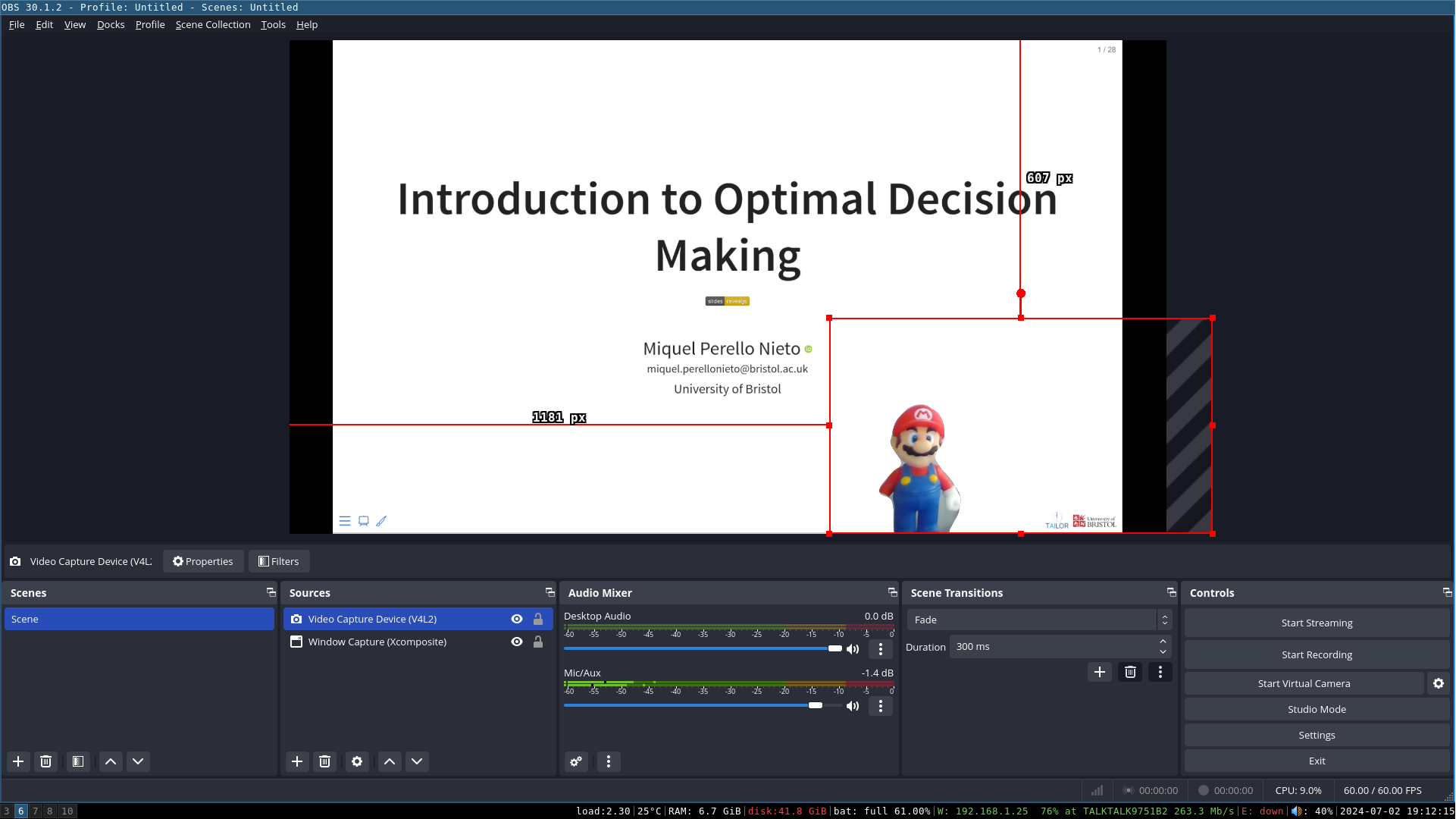
The video recordings required the accompanying set of slides generated from the same course. Given that the slides contain a reduced version of the website, it is possible to create the slides and the videos before the narrative is finalised, which has been the approach taken for this course. The video were recorded in a home environment with non-professional devices such as a common laptop and its internal microphone. In order to record both the slides and the speaker we used OBS (Open Bradcaster Software) Studio which is a free and open-source software for video recording (and live streaming) available for Windows, Mac and Linux.
The background of the speaker was removed using an OBS Studio plugin that does not require a green screen . However, the parameters need to be adjusted which can affect the computation cost and the precision of the background removal. For online courses it is recommended to create short videos of a very specific topic (less than 10 minutes) to facilitate the time management of the students, and to potentially reuse some video recordings in similar courses. A total of four videos were recorded with an average length of approximately 9 minutes. The videos are currently hosted on YouTube and can be used without the other content.

Fig. 4 OBS Studio configured to record the set of slides and video capture with a plugin that automatically removes the background.#
In order to install the background removal plugin in Ubuntu 20.04 it is
necessary to install OBS and the plugin from flatpak with the following
commands:
flatpak remote-add --if-not-exists flathub https://flathub.org/repo/flathub.flatpakrepo
flatpak install flathub com.obsproject.Studio
flatpak install flathub com.obsproject.Studio.Plugin.BackgroundRemoval
The following video is an example of the results obtained using the reveal.js
slides generated with Quarto and the video recorded with OBS and the
automatic removal of the background.
