Dynamic content#
Dynamic content is content that includes computational code that is
executed when the website/book is built. With extra configurations, the content
can be re-run in real time locally or with a third party service like MyBiner,
Google Colab, or others. This type of content is very useful for educational
material in science, technology, engineering and mathematics. Jupyter Notebooks
and other programming environments that integrate a textual narrative,
computational cells and their results are really common. Publishing systems
like Jupyter Book and Quarto support multiple ways to write this type of
material by using directives (See Roles and Directives) for code in markdown files, or
directly using Jupyter Notebooks. This section serves as an example of the
functionalities that can be integrated in a Markdown file in a Jupyter Book. We
also indicate what are the differences in the Quarto publishing system when
necessary.
Configuration#
Adding dynamic content that changes during the execution requires the specification of a kernel which is able to read the code indicated in the apropiate directives and produce an ouptut result. This configuration differs slighly depending on the platform and the type of file (e.g. markdown and Jupyter Notebook).
Jupyter Notebook files#
Jupyter Notebooks are web-based documents that combine a textual narrative
(written in a markup language) with computational elements (supporting a
multitude of programming languages). The code of the notebooks can be executed
with the help of a
kernel; a
programming language specific process that can interpret the code, run it and
provide the results to the authoring application. The default kernel is the
ipykernel built on top of
IPython. Common functionalities added via the code
cells are the generation of figures, tables, plots, and interactive elements
and the analysis of data. Jupyter Notebooks have a file extension .ipynb and
can be edited with authoring tools like Jupyter Notebook, Jupyter Lab,
Google Colab, and most integrated development environments (IDEs) like
PyCharm, Microsoft Visual Studio, Posit, and RStudio (See also Computational notebook editors).
In Jupyter Book and Quarto projects the configuration of Jupyter Notebooks is general across the project. However, Quarto requires a Raw
cell at the beginning of the notebook with the title, author, and any
additional options that you want to include in order to be rendered. The
following is a configuration example for Quarto:
---
title: Title of the page
authors: "Miquel Perello Nieto"
date: "July 11th, 2024"
format:
  html: default
  pdf: default
  refealjs: default
---
Markdown files#
In Jupyter Book, Markdown files with dynamic content require a YAML
configuration in the header indicating some parameters about
the type of file and the kernel to use. There are kernels for different
programming languages like R, Python, Julia, and more. For example, the
markdown file for this page has been configured to run Python3 with the
following yaml configuration
---
jupytext:
  cell_metadata_filter: -all
  formats: md:myst
  text_representation:
    extension: .md
    format_name: myst
    format_version: 0.13
    jupytext_version: 1.11.5
kernelspec:
  display_name: Python 3
  language: python
  name: python3
---
The header can be generated automatically with the help of the jupyter-book
tool by running the following command in a terminal at the root of the project
jupyter-book myst init markdownfile.md --kernel kernelname
Additional documentation can be found at https://jupyterbook.org/en/stable/file-types/myst-notebooks.html.
Running Python code in the Quarto publishing system requires the jupyter
Python package and the specification of the python command to use in the
YAML header or in the _quarto.yml configuration file.
jupyter: python3
Live code#
In Jupyter Book, Thebe offers a
solution to launch the kernel in the current page (without the need to jump to
a third party website).
The web page you are currently reading has been configured to
run Thebe with the third party service MyBinder. This was achieved by adding
the following line of code before the first title of the markdown document:
(launch:thebe)=
The top of the page now displays the spaceship icon.
You can launch Thebe by clicking on it and select Live code in the
drop down menu:

Fig. 2 Menu to launch Live Code with Thebe#
This will launch the code in your configured server (in this case MyBinder) and a new loading text will be shown at the top of the current page with several steps, building the code, publishing and launching. Depending on the configured server this process may take some time to complete, and occasionally could fail to launch.
Fig. 3 Steps that Live Code will show as it prepares the running environment.#
Once the kernel is ready, any Python code that is written in a {code-cell}
with ipython3 can be modified and re-run in real time.
The current page is an example in which you can modify all the cells.
Quarto does not currently support Thebe, but it supports launching the
code in a third party environment like MyBinder by adding the following
yaml configuration in the header of the Markdown file
code-links: binder
Quarto has good integration with Shiny which has
additional functionalities that can bee seen in Section Interactive content.
Simple examples#
In Jupyter Books by using the code-cell directive it is possible to execute
code and print out its response.
```{code-cell}
print("Hello world!")
```
When your book is being built, the contents of any {code-cell} block will be
executed with the default Jupyter kernel. The outputs will be displayed in-line
with the rest of your content.
print("2 + 2 = ", 2 + 2)
2 + 2 = 4
It is possible to modify the behaviour of code-cells by adding tags. For
example the tag hide-input will make the code hidden until it is clicked with
the mouse.
```{code-cell} ipython3
:tags: [hide-input, thebe-init]

# Python code
```
The following code is an example:
Show code cell source
import numpy as np

np.random.seed(42)

hidden_text = f"The result of this draw of a six sided dice is {np.random.randint(1, 6)}"
The previous example generates a random number between 1 and 6 and stores the result in a variable. The content of the variable can be printed in a separate cell
print(hidden_text)
The result of this draw of a six sided dice is 4
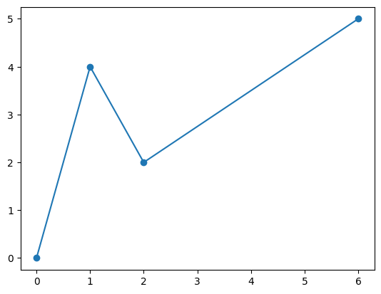
The following code illustrates how to create a lineplot which can be easily modified in a Live environment.
import matplotlib.pyplot as plt

plt.plot([0, 1, 2, 6], [0, 4, 2, 5], 'o-')
[<matplotlib.lines.Line2D at 0x7ff5c01f8d90>]

Exploration of tables#
In data analysis it is common to inspect large amounts of data which in certain
cases is stored in a tabular form. Pandas is a Python library that is able to
produce Data Frames (similar to the Data Frames from the R programming
language), and can produce summaries and visualisations in various output
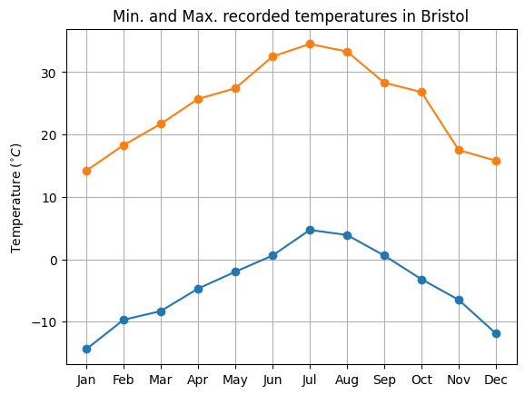
formats. The following example shows the recorded temperatures (Celsius) in
Bristol as shown in its Wikipedia article1.
import pandas

features = ['Record low', 'Record high']
date = ['Jan', 'Feb', 'Mar', 'Apr', 'May', 'Jun', 'Jul', 'Aug', 'Sep', 'Oct',
        'Nov', 'Dec']
data = [[-14.4, 14.2], [-9.7, 18.3], [-8.3, 21.7], [-4.7, 25.7], [-2.0, 27.4],
        [0.6, 32.5], [4.7, 34.5], [3.9, 33.3], [0.6, 28.3], [-3.2, 26.8],
        [-6.5, 17.5], [-11.9, 15.8]]
df = pandas.DataFrame(data=data, index=date, columns=features)

df.style.background_gradient(cmap='coolwarm', vmin=df.min().min(), vmax=df.max().max())
| Record low | Record high | |
|---|---|---|
| Jan | -14.400000 | 14.200000 |
| Feb | -9.700000 | 18.300000 |
| Mar | -8.300000 | 21.700000 |
| Apr | -4.700000 | 25.700000 |
| May | -2.000000 | 27.400000 |
| Jun | 0.600000 | 32.500000 |
| Jul | 4.700000 | 34.500000 |
| Aug | 3.900000 | 33.300000 |
| Sep | 0.600000 | 28.300000 |
| Oct | -3.200000 | 26.800000 |
| Nov | -6.500000 | 17.500000 |
| Dec | -11.900000 | 15.800000 |
The cells are not independent, and following computations can be performed making reference to variables instantiated in previous cells. The following example shows some statistics of the previous table.
df.describe()
| Record low | Record high | |
|---|---|---|
| count | 12.000000 | 12.000000 |
| mean | -4.241667 | 24.666667 |
| std | 6.124831 | 7.056568 |
| min | -14.400000 | 14.200000 |
| 25% | -8.650000 | 18.100000 |
| 50% | -3.950000 | 26.250000 |
| 75% | 0.600000 | 29.350000 |
| max | 4.700000 | 34.500000 |
Static plots#
Figures generated with plotting libraries can also be rendered and shown as static images (e.g. matplotlib, pyplot, bokeh). The following is an example with the previous temperatures rendered with `Matplotlib``.
import matplotlib.pyplot as plt
plt.plot(df, '-o')
plt.ylabel('Temperature ($^{\circ}C$)')
plt.title('Min. and Max. recorded temperatures in Bristol')
plt.grid()

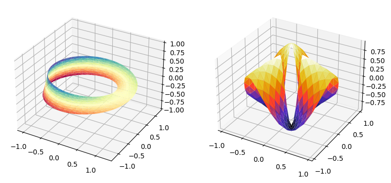
Or the following examples of 3D surfaces from the Matplotlib documentation.
from bpython.examples import matplotlib_trisurf3d_2

matplotlib_trisurf3d_2()

Code listing#
It is possible to print the source code of any Python function with the package
inspect. The following is an example for a function in the bpython package.
def function_example(a: float, b: float):
    """Sums two numbers

    Parameters
    ----------
    a : float
      First number to sum
    b : float
      Second number to sum
    """
    return a + b
Then it is possible to get the function documentation
import inspect

documentation = inspect.getdoc(function_example)
print(documentation)
Sums two numbers

Parameters
----------
a : float
  First number to sum
b : float
  Second number to sum
or its source code
source = inspect.getsource(function_example)
print(source)
def function_example(a: float, b: float):
    """Sums two numbers

    Parameters
    ----------
    a : float
      First number to sum
    b : float
      Second number to sum
    """
    return a + b
Reuse of complex code#
In order to reuse complex code across the website, it is recommended to write a
package with the functions. In the case of the current roadmap, we have created
a package bpython in the folder
/lib/book-python/.
It can be installed after the requirements with
pip install -e /lib/book-python/
The -e option keeps the library in its current folder, allowing the
modification of the library during the development of the website. In this way,
every time that the virtual environment is loaded the library is loaded anew.
The following code should print the current version of this auxiliary library.
import bpython

print(f"The current BPython version is {bpython.__version__}")
The current BPython version is 0.0.1.dev1
Another example with a complex 3D surface visualisation from the Matplotlib documentation was already shown in Section Static plots.
