Introduction to Optimal Decision Making

Miquel Perello Nieto

miquel.perellonieto@bristol.ac.uk

University of Bristol

Motivation

Optimal Decision Making. Why and how?

The objective is to classify a new instance into one of the possible classes in an optimal manner.
This may be important in critical applications: e.g. medical diagnosis (Begoli, Bhattacharya, and Kusnezov 2019; Yang, Steinfeld, and Zimmerman 2019), self-driving cars (Qayyum et al. 2020; Mullins et al. 2018), extreme weather prediction, finances (Nti, Adekoya, and Weyori 2020).
It is necessary to know what are the consequences of making each prediction (costs or gains).
One way to make optimal decisions is with cost-sensitive classification.
Can we make optimal decisions with any type of classifier?

Optimal decisions with different types of model

Class estimation: Outputs a class prediction.
Class estimation with option of abstaining: Outputs a class prediction or abstains (Coenen, Abdullah, and Guns 2020; Mozannar and Sontag 2020)
Rankings estimation: Outputs a ranked list of possible classes (Brinker and Hüllermeier 2020).
Score surrogates: Outputs a continuous score which is commonly a surrogate for classification (e.g. Support Vector Machines).
Probability estimation: Outputs class posterior probability estimates (e.g. Logistic Regression, naive Bayes, Artificial Neural Networks), or provides class counts which can be interpreted as proportions (e.g. decision trees, random forests, k-nearest neightbour) (Zadrozny and Elkan 2001).
Other types of outputs: Some examples are possibility theory (Dubois and Prade 2001), credal sets (Levi 1980), conformal predictions (Vovk, Gammerman, and Shafer 2005), multi-label (Alotaibi and Flach 2021).

Cost-sensitive classification

Cost-sensitive classification (Elkan 2001) provides a framework to make optimal decisions (with certain assumptions).
We require the true posterior probabilities of each outcome in order to make optimal decisions, but we can use estimates.
Assumes the costs are not instance dependent (only depend on the predicted and true class).
Class priors and costs can be changed during deployment (if known or estimated).

Cost matrices: Binary example

The following is a typical example of a cost matrix \(c\) for a binary problem.

	Predicted \(C_1\)	Predicted \(C_2\)
True \(C_1\)	\(\color{DarkGreen}{0}\)	\(\color{DarkRed}{1}\)
True \(C_2\)	\(\color{DarkRed}{1}\)	\(\color{DarkGreen}{0}\)

We will refer to \(c_{i|j}\) the cost of predicting class \(C_i\) given that the true class is \(C_j\).

Given the posterior probabilities \(P(C_j|\mathbf{x})\) where \(j \in \{1, K\}\) and the cost matrix \(c\) we can calculate the expected cost of predicting class \(C_i\)

\[\begin{equation} \mathbb{E}_{j \sim P(\cdot|\mathbf{x})} (c_{i|j}) = \sum_{j = 1}^K P(C_j|\mathbf{x}) c_{i|j}. \end{equation}\]

For example, lets assume that the posterior probability vector for a given instance is \([0.4, 0.6]\), the expected costs will be

Predicting Class 1 will have an expected cost of \(0.4 \times 0 + 0.6 \times 1 = \color{DarkRed}{0.6}\)
Predicting Class 2 will have an expected cost of \(0.4 \times 1 + 0.6 \times 0 = \mathbf{\color{DarkRed}{0.4}}\).

Expected costs figure

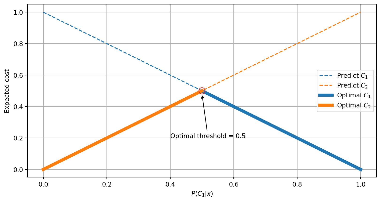
We can visualise the cost lines for each prediction with a line for each predicted class \(C_i\) and its missclassification costs and correct predictions (Drummond and Holte 2006). For example, the following cost matrix

	Predicted \(C_1\)	Predicted \(C_2\)
True \(C_1\)	\(\color{DarkGreen}{0}\)	\(\color{DarkRed}{1}\)
True \(C_2\)	\(\color{DarkRed}{1}\)	\(\color{DarkGreen}{0}\)

will result in the following cost lines

where we have highlighted the minimum cost among the possible predictions. In this particular case the optimal prediction changes when the probability of the true class is higher or lower than \(0.5\), with the same expected cost for both classes at \(0.5\).

Cost Matrix “reasonableness” condition

In general, it is reasonable to expect cost matrices where:

For a given class \(j\) the correct prediction has always a lower cost than an incorrect prediction \(c_{j|j} < c_{i|j}\) with \(i \neq j\).
Class domination: One class does not consistently have lower costs than other classes \(c_{i|j} \leq c_{k|j}\) for all \(j\).

We will make these reasonable assumptions in this introductory module.

Class Domination

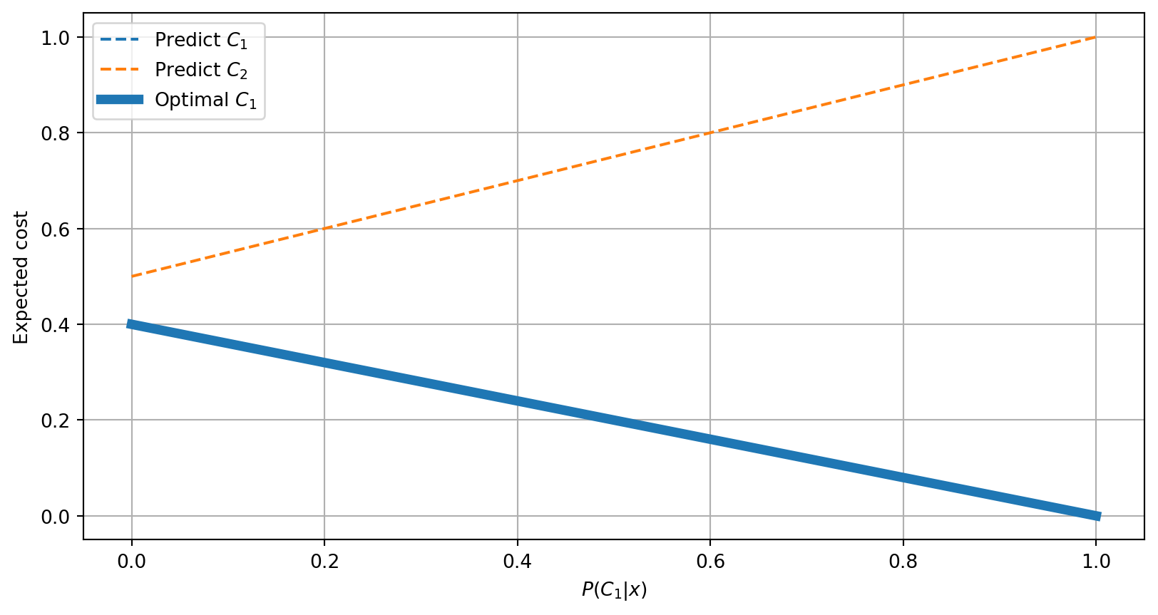
The following is an example of class domination in which predicting class \(C_1\) will always have a lower expected cost.

	Predicted \(C_1\)	Predicted \(C_2\)
True \(C_1\)	\(\color{DarkGreen}{0}\)	\(\color{DarkRed}{1}\)
True \(C_2\)	\(\color{DarkRed}{0.4}\)	\(\color{DarkGreen}{0.5}\)

Optimal threshold for the binary case

If we know the true posterior probabilities, the optimal decision is to choose the class that minimizes the expected cost which can be obtained by marginalising the predicted class over all possible true classes (O’Brien, Gupta, and Gray 2008).

\[\begin{equation} \hat{y}(\mathbf{x}) = \mathop{\mathrm{arg\,min}}_{i=\{1, \dots, K\}} \mathbb{E}_{j \sim P(\cdot|\mathbf{x})} (c_{i|j}) = \mathop{\mathrm{arg\,min}}_{i=\{1, \dots, K\}} \sum_{j=1}^K P(C_j|\mathbf{x}) c_{i|j}. \end{equation}\]

In the binary case we want to predict class \(C_1\) if and only if predicting class \(C_1\) has a lower expected cost than predicting class \(C_2\)

\[\begin{align} \sum_{j=1}^K P(C_j|\mathbf{x}) c_{1|j} &\le \sum_{j=1}^K P(C_j|\mathbf{x}) c_{2|j} \\ P(C_1|\mathbf{x}) c_{1|1} + P(C_2|\mathbf{x}) c_{1|2} &\le P(C_1|\mathbf{x}) c_{2|1} + P(C_2|\mathbf{x}) c_{2|2} \\ \end{align}\]

with the equality having the same expected cost independent on the predicted class.

\[\begin{equation} p c_{1|1} + (1 - p) c_{1|2} = p c_{2|1} + (1 - p) c_{2|2} \end{equation}\]

where \(p = P(C_1|\mathbf{x})\).

In the binary classification setting we can derive the optimal threshold \(t^*\) of selecting class one if \(p \ge t^*\).

\[\begin{align} t^* c_{1|1} + (1 - t^*) c_{1|2} &= t^* c_{2|1} + (1 - t^*) c_{2|2} \\ (1 - t^*) c_{1|2} - (1 - t^*) c_{2|2} &= t^* c_{2|1} - t^* c_{1|1} \\ (1 - t^*) (c_{1|2} - c_{2|2}) &= t^* (c_{2|1} - c_{1|1}) \\ (c_{1|2} - c_{2|2}) -t^*(c_{1|2} - c_{2|2}) &= t^* (c_{2|1} - c_{1|1}) \\ (c_{1|2} - c_{2|2}) &= t^* (c_{2|1} - c_{1|1}) + t^*(c_{1|2} - c_{2|2}) \\ (c_{1|2} - c_{2|2}) &= t^* (c_{2|1} - c_{1|1} + c_{1|2} - c_{2|2}) \\ \frac{c_{1|2} - c_{2|2}}{c_{2|1} - c_{1|1} + c_{1|2} - c_{2|2}} &= t^* \end{align}\]

For the previous cost matrix

	Predicted \(C_1\)	Predicted \(C_2\)
True \(C_1\)	\(\color{DarkGreen}{0}\)	\(\color{DarkRed}{1}\)
True \(C_2\)	\(\color{DarkRed}{1}\)	\(\color{DarkGreen}{0}\)

the optimal threshold corresponds to

\[\begin{equation} t^* = \frac{{\color{DarkRed}c_{1|2}} - {\color{DarkGreen}c_{2|2}}} {{\color{DarkRed}c_{1|2}} - {\color{DarkGreen}c_{2|2}} + {\color{DarkRed}c_{2|1}} - {\color{DarkGreen}c_{1|1}}} = \frac{1 - 0}{1 + 1 - 0 - 0} = 0.5 \end{equation}\]

Different costs binary example

In general, the correct predictions have a cost of \(0\). However, this may be different in certain scenarios. The following is an example of a cost matrix with different gains on the main diagonal and missclassification costs.

	Predicted \(C_1\)	Predicted \(C_2\)
True \(C_1\)	\(\color{DarkGreen}{-5}\)	\(\color{DarkRed}{10}\)
True \(C_2\)	\(\color{DarkRed}{1}\)	\(\color{DarkGreen}{-1}\)

which would result in the following cost lines.

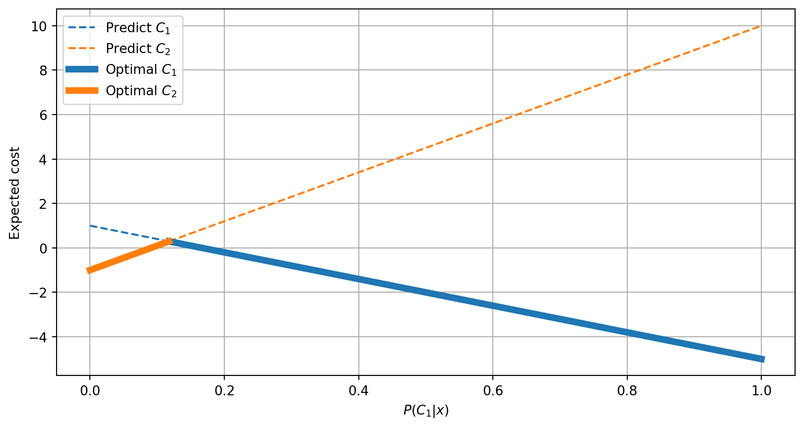
In this case, for a posterior probability vector \([0.4, 0.6]\) we would expect

Predicting Class 1 will have an expected cost of \(-5 \times 0.4 + 1 \times 0.6 = \mathbf{\color{DarkGreen}{-1.4}}\)
Predicting Class 2 will have an expected cost of \(10 \times 0.4 - 1 \times 0.6 = \color{DarkRed}{3.4}\)

Other binary examples

See how the beginning and end of the cost lines change with the costs.

#| standalone: true
#| components: viewer
#| viewerHeight: 480

import matplotlib.pyplot as plt
from shiny import App, render, ui
import pandas as pd

app_ui = ui.page_fluid(
    ui.layout_sidebar(
        ui.sidebar(
    ui.input_slider("TP", "Cost True C1",  value=-5, min=-10, max=0),
    ui.input_slider("TN", "Cost True C2",  value=-1, min=-10, max=0),
    ui.input_slider("FN", "Cost False C2", value=10, min=1,   max=10),
    ui.input_slider("FP", "Cost False C1", value=1,  min=1,   max=10),
    ),
    ui.output_plot("plot")
    ),
)

def server(input, output, session):
    @output
    @render.plot(alt="A histogram")
    def plot():
        TP = input.TP() # C_1|1
        FN = input.FN() # C_1|2
        FP = input.FP() # C_2|1
        TN = input.TN() # C_2|2
        fig = plt.figure()
        ax = fig.add_subplot()
        ax.grid(True)
        ax.plot([0, 1], [FP, TP], '--', label="Predict $C_1$")
        ax.plot([0, 1], [TN, FN], '--', label="Predict $C_2$")

        threshold = (FP - TN)/(FP - TN + FN - TP)
        cost_t = threshold*TP + (1-threshold)*FP
        ax.plot([threshold, 1], [cost_t, TP], lw=5, color='tab:blue', label="Optimal $C_1$")
        ax.plot([0, threshold], [TN, cost_t], lw=5, color='tab:orange', label="Optimal $C_2$")

        C = [[TP, FP], [FN, TN]]
        bbox = dict(boxstyle="round", fc="white")
        ax.annotate(r'$C_{2|2}$', (0, C[1][1]), xytext=(2, -1),
                    textcoords='offset fontsize',
                    arrowprops=dict(arrowstyle='->', facecolor='black'),
                    bbox=bbox)
        ax.annotate(r'$C_{1|1}$', (1, C[0][0]), xytext=(2, 0),
                    textcoords='offset fontsize',
                    arrowprops=dict(arrowstyle='->', facecolor='black'),
                    bbox=bbox)
        ax.annotate(r'$C_{1|2}$', (0, C[0][1]), xytext=(0, 2),
                    textcoords='offset fontsize',
                    arrowprops=dict(arrowstyle='->', facecolor='black'),
                    bbox=bbox)
        ax.annotate(r'$C_{2|1}$', (1, C[1][0]), xytext=(2, 0),
                    textcoords='offset fontsize',
                    arrowprops=dict(arrowstyle='->', facecolor='black'),
                    bbox=bbox)

        ax.annotate(f'$t*={threshold:0.2}$', (threshold, cost_t), 
                    xytext=(0, --3),
                    textcoords='offset fontsize',
                    arrowprops=dict(arrowstyle='->', facecolor='black'),
                    bbox=bbox)

        ax.set_xlabel('$P(C_1|x)$')
        ax.set_ylabel('Expected cost')
        ax.legend()

        return fig

app = App(app_ui, server, debug=True)

Cost invariances

The optimal prediction does not change if the cost matrix is

Multiplied by a positive constant value
Shifted by a constant value

#| standalone: true
#| components: viewer
#| viewerHeight: 480

import numpy as np
import matplotlib.pyplot as plt
from shiny import App, render, ui
import pandas as pd


def fraction_to_float(fraction):
    if '/' in fraction:
       numerator, denominator = fraction.split('/') 
       result = float(numerator)/float(denominator)
    else:
       result = float(fraction)
    return result

# X|Y means predict X given that the true label is Y
# Because the indices in a matrix are first row and then column we need to
# invert the order of X and Y by transposing the matrix. Then [0,1] is predict 0
# when the true label is 1.
# TODO: check indices
C_original = np.array([[-2,  3],     # 1|1, 2|1
                       [13, -7]]).T  # 1|2, 2|2

app_ui = ui.page_fluid(
    ui.layout_sidebar(
        ui.sidebar(
            ui.input_slider("S", "Shift constant S", value=0,  min=-10,
                            max=10),
            ui.input_radio_buttons("M", "Multiplicative constant M",
                                   choices=['1/20', '1/10', '1/5', '1',
                                            '5', '10', '20'],
                                   selected = '1', inline=True, width='100%'),
            ui.output_table('cost_matrix'),
        ),
        ui.output_plot("plot")
    ),
)

def server(input, output, session):
    @output
    @render.plot(alt="A histogram")
    def plot():
        fig = plt.figure()
        ax = fig.add_subplot()
        ax.grid(True)

        global C_original
        C = C_original + input.S()
        C = C*fraction_to_float(input.M())
        
        threshold = (C[0][1] - C[1][1])/(C[0][1] - C[1][1] + C[1][0] - C[0][0])
        cost_t = threshold*C[0][0] + (1-threshold)*C[0][1]

        ax.plot([0, 1], [C[0][1], C[0][0]], '--', label="Predict $C_1$")
        ax.plot([0, 1], [C[1][1], C[1][0]], '--', label="Predict $C_2$")
        ax.plot([threshold, 1], [cost_t, C[0][0]], lw=5, color='tab:blue', label="Optimal $C_1$")
        ax.plot([0, threshold], [C[1][1], cost_t], lw=5, color='tab:orange', label="Optimal $C_2$")

        bbox = dict(boxstyle="round", fc="white")
        ax.annotate(r'$C_{2|2}$', (0, C[1][1]), xytext=(-0.2, C[1][1]),
                    arrowprops=dict(arrowstyle='->', facecolor='black'),
                    bbox=bbox)
        ax.annotate(r'$C_{1|1}$', (1, C[0][0]), xytext=(1.1, C[0][0]),
                    arrowprops=dict(arrowstyle='->', facecolor='black'),
                    bbox=bbox)
        ax.annotate(r'$C_{1|2}$', (0, C[0][1]), xytext=(-0.2, C[0][1]),
                    arrowprops=dict(arrowstyle='->', facecolor='black'),
                    bbox=bbox)
        ax.annotate(r'$C_{2|1}$', (1, C[1][0]), xytext=(1.1, C[1][0]),
                    arrowprops=dict(arrowstyle='->', facecolor='black'),
                    bbox=bbox)

        ax.annotate(f'$t*={threshold:0.2}$', (threshold, cost_t), 
                    xytext=(threshold + 0.2, cost_t),
                    arrowprops=dict(arrowstyle='->', facecolor='black'),
                    bbox=bbox)

        ax.set_xlabel('$P(C_1|x)$')
        ax.set_ylabel('Expected cost')
        ax.legend()

        return fig
    @output
    @render.table(index=True)
    def cost_matrix():
        global C_original
        C = C_original.T + input.S() # Need to transpose back to show print matrix
        C = C*fraction_to_float(input.M())

        return pd.DataFrame(C,
                            index=['True C1', 'True C2'],
                            columns=['Predicted C1', 'Predicted C2'])

app = App(app_ui, server, debug=True)

Simplification example

Because of these invariances, it is common in the binary case to modify the matrix \(c\) in such a way that the missclassification cost for one of the classes is \(1\) and a cost of \(0\) for its correct prediction. For example, if \(c_{1|2}^*=1\) and \(c_{2|2}^*=0\) we get

In the previous example the original cost matrix \(c\)

\[\begin{equation} c = \begin{bmatrix}-2 & 3 \\ 13 & -7\end{bmatrix}^\intercal \end{equation}\]

if shifted by \(+7\) and scaled by \(1/20\) results in

\[\begin{equation} c' = \begin{bmatrix} (-2 + 7)/20 & (3 + 7)/20 \\ (13 + 7)/20 & (-7 + 7)/20\end{bmatrix}^\intercal = \begin{bmatrix}0.25 & 0.5 \\ 1 & 0\end{bmatrix}^\intercal \end{equation}\]

with an optimal threshold

\[\begin{equation} t^* = \frac{1} {1 + {\color{DarkRed}c_{2|1}}' - {\color{DarkGreen}c_{1|1}'}} = \frac{1} {1 + {\color{DarkRed}0.5} - {\color{DarkGreen}0.25}} = 0.8 \end{equation}\]

Multiclass setting

The binary cost matrix can be extended to multiclass by extending the rows with additional true classes and columns with predicted classes.

	Predicted \(C_1\)	Predicted \(C_2\)	\(\cdots\)	Predicted \(C_K\)
True \(C_1\)	\(\color{DarkGreen}{c_{1\|1}}\)	\(\color{DarkRed}{c_{2\|1}}\)	\(\cdots\)	\(\color{DarkRed}{c_{K\|1}}\)
True \(C_2\)	\(\color{DarkRed}{c_{1\|2}}\)	\(\color{DarkGreen}{c_{2\|2}}\)	\(\cdots\)	\(\color{DarkRed}{c_{2\|2}}\)
\(\vdots\)	\(\vdots\)	\(\vdots\)	\(\ddots\)	\(\vdots\)
True \(C_K\)	\(\color{DarkRed}{c_{1\|K}}\)	\(\color{DarkRed}{c_{2\|K}}\)	\(\cdots\)	\(\color{DarkGreen}{c_{K\|K}}\)

However, with more than 2 classes the threshold is not a single value but multiple decision boundaries in the probability simplex.

Ternary example {.smaller}

In order to exemplify the process of making an optimal decision in more with more than two classes we can look at the ternary case, which naturally extends to more classes. Given the following cost matrix

	Predicted \(C_1\)	Predicted \(C_2\)	Predicted \(C_3\)
True \(C_1\)	\(\color{DarkGreen}{-10}\)	\(\color{DarkRed}{20}\)	\(\color{DarkRed}{30}\)
True \(C_2\)	\(\color{DarkRed}{40}\)	\(\color{DarkGreen}{-50}\)	\(\color{DarkRed}{60}\)
True \(C_3\)	\(\color{DarkRed}{70}\)	\(\color{DarkRed}{80}\)	\(\color{DarkGreen}{-90}\)

and a true posterior probability vector for all the classes \([0.5, 0.1, 0.4]\), we can estimate the expected cost of making each class prediction

\[\begin{equation} \mathbb{E}_{j \sim P(\cdot|\mathbf{x})} (c_{i|j}) = \sum_{j = 1}^K P(C_j|\mathbf{x}) c_{i|j}. \end{equation}\]

which results in the following expected costs:

Predicting Class 1 will have a cost of \(-10 \times 0.5 + 40 \times 0.1 +70 \times 0.4 = \color{DarkRed}{27}\)
Predicting Class 2 will have a cost of \(20 \times 0.5 - 50 \times 0.1 +80 \times 0.4 = \color{DarkRed}{37}\)
Predicting Class 3 will have a cost of \(30 \times 0.5 + 60 \times 0.1 -90 \times 0.4 = \mathbf{\color{DarkGreen}{-15}}\)

Ternary expected cost isolines per decision

	Predicted \(C_1\)	Predicted \(C_2\)	Predicted \(C_3\)
True \(C_1\)	\(\color{DarkGreen}{-10}\)	\(\color{DarkRed}{20}\)	\(\color{DarkRed}{30}\)
True \(C_2\)	\(\color{DarkRed}{40}\)	\(\color{DarkGreen}{-50}\)	\(\color{DarkRed}{60}\)
True \(C_3\)	\(\color{DarkRed}{70}\)	\(\color{DarkRed}{80}\)
\(\color{DarkGreen}{-90}\)

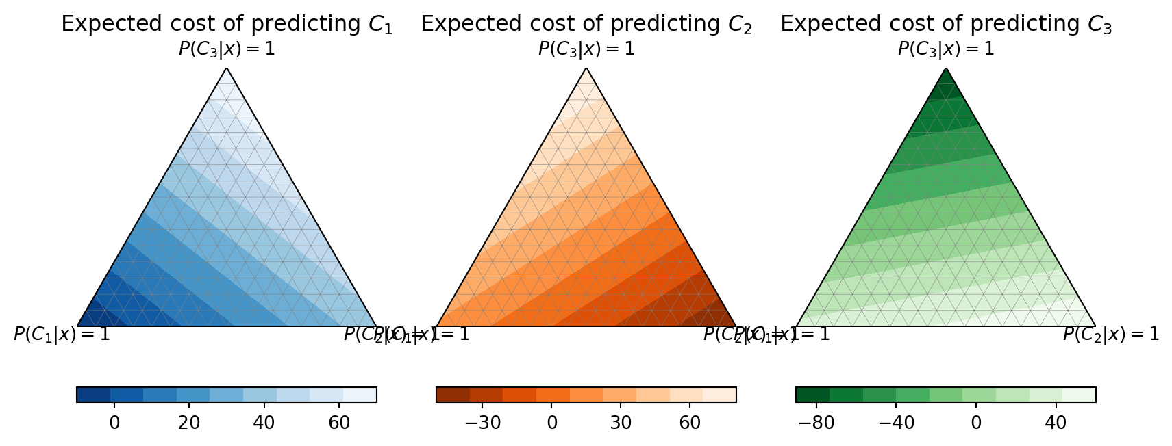
Ternary hyperplanes optimal decision combined

	Predicted \(C_1\)	Predicted \(C_2\)	Predicted \(C_3\)
True \(C_1\)	\(\color{DarkGreen}{-10}\)	\(\color{DarkRed}{20}\)	\(\color{DarkRed}{30}\)
True \(C_2\)	\(\color{DarkRed}{40}\)	\(\color{DarkGreen}{-50}\)	\(\color{DarkRed}{60}\)
True \(C_3\)	\(\color{DarkRed}{70}\)	\(\color{DarkRed}{80}\)
\(\color{DarkGreen}{-90}\)

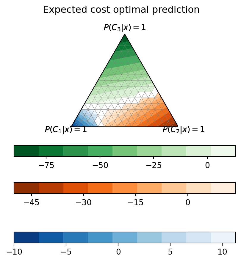
Option to abstain

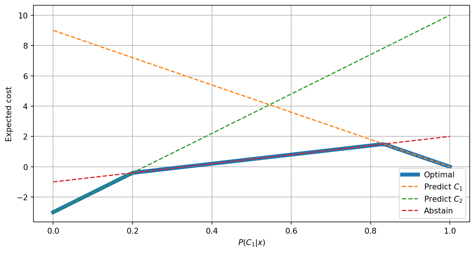
It is possible to add the costs of abstaining on making a prediction by adding a column into the original cost matrix (Charoenphakdee et al. 2021). The following is an example which illustrates this in a binary classification problem.

	Predicted \(C_1\)	Predicted \(C_2\)	Abstain
True \(C_1\)	\(\color{DarkGreen}{0}\)	\(\color{DarkRed}{10}\)	\(\color{DarkRed}{2}\)
True \(C_2\)	\(\color{DarkRed}{9}\)	\(\color{DarkGreen}{-3}\)	\(\color{DarkRed}{2}\)

Predicting Class 1 has an expected cost of \(0 \times 0.3 + 9 \times 0.7 = \color{DarkRed}{6.3}\)
Predicting Class 2 has an expected cost of \(10 \times 0.3 - 3 \times 0.7 = \mathbf{\color{DarkRed}{0.9}}\)
Abstaining has an expected cost of \(2 \times 0.3 + 2 \times 0.7 = \color{DarkRed}{2}\)

Option to abstain cost lines

	Predicted \(C_1\)	Predicted \(C_2\)	Abstain
True \(C_1\)	\(\color{DarkGreen}{0}\)	\(\color{DarkRed}{10}\)	\(\color{DarkRed}{2}\)
True \(C_2\)	\(\color{DarkRed}{9}\)	\(\color{DarkGreen}{-3}\)	\(\color{DarkRed}{2}\)

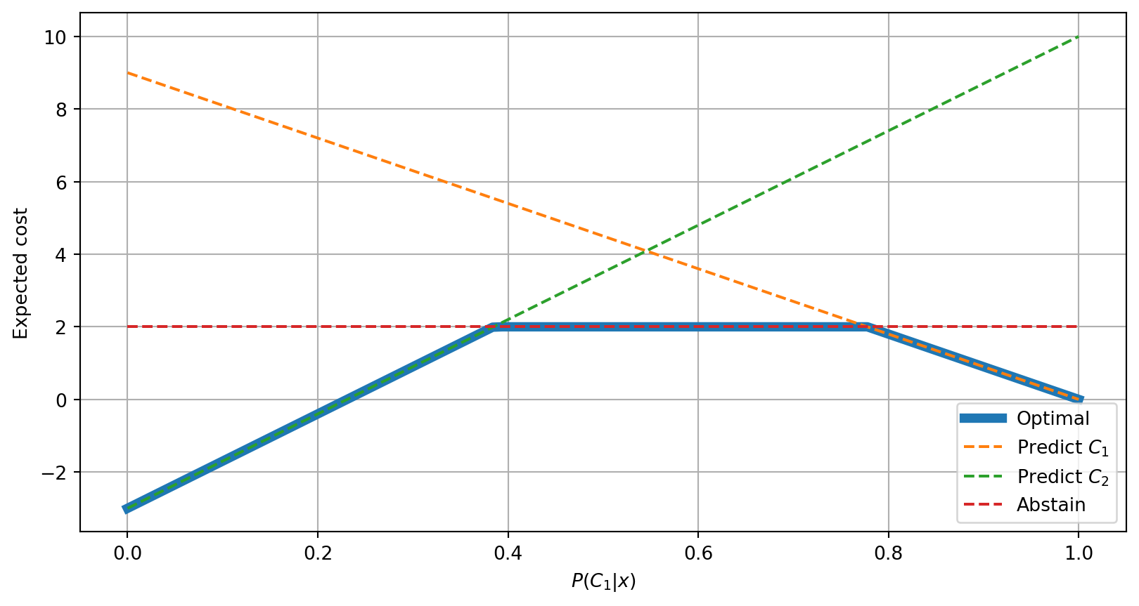
Option to abstain different costs

The following is another example in which abstaining from making a prediction if the true class was \(C_2\) would incur into a gain.

	Predicted \(C_1\)	Predicted \(C_2\)	Abstain
True \(C_1\)	\(\color{DarkGreen}{0}\)	\(\color{DarkRed}{10}\)	\(\color{DarkRed}{2}\)
True \(C_2\)	\(\color{DarkRed}{9}\)	\(\color{DarkGreen}{-3}\)	\(\color{DarkGreen}{-1}\)

References

Alotaibi, Reem, and Peter Flach. 2021. “Multi-Label Thresholding for Cost-Sensitive Classification.” Neurocomputing 436 (May): 232–47. https://doi.org/10.1016/J.NEUCOM.2020.12.004.

Begoli, Edmon, Tanmoy Bhattacharya, and Dimitri Kusnezov. 2019. “The Need for Uncertainty Quantification in Machine-Assisted Medical Decision Making.” Nature Machine Intelligence 1 (1): 20–23.

Brinker, Klaus, and Eyke Hüllermeier. 2020. “A Reduction of Label Ranking to Multiclass Classification.” In Machine Learning and Knowledge Discovery in Databases: European Conference, ECML PKDD 2019, würzburg, Germany, September 16–20, 2019, Proceedings, Part III, 204–19. Springer.

Charoenphakdee, Nontawat, Zhenghang Cui, Yivan Zhang, and Masashi Sugiyama. 2021. “Classification with Rejection Based on Cost-Sensitive Classification.” In Proceedings of the 38th International Conference on Machine Learning, edited by Marina Meila and Tong Zhang, 139:1507–17. PMLR. https://proceedings.mlr.press/v139/charoenphakdee21a.html http://arxiv.org/abs/2010.11748.

Coenen, Lize, Ahmed KA Abdullah, and Tias Guns. 2020. “Probability of Default Estimation, with a Reject Option.” In 2020 IEEE 7th International Conference on Data Science and Advanced Analytics (DSAA), 439–48. IEEE.

Drummond, Chris, and Robert C. Holte. 2006. “Cost curves: An improved method for visualizing classifier performance.” Machine Learning 65 (1): 95–130.

Dubois, Didier, and Henri Prade. 2001. “Possibility Theory, Probability Theory and Multiple-Valued Logics: A Clarification.” Annals of Mathematics and Artificial Intelligence 32: 35–66.

Elkan, Charles. 2001. “The Foundations of Cost-Sensitive Learning The Foundations of Cost-Sensitive Learning.” In 17th International Conference on Artificial Intelligence (IJCAI’01), edited by Morgan Kaufmann, 973—–978. May 2001.

Levi, Isaac. 1980. The Enterprise of Knowledge: An Essay on Knowledge, Credal Probability, and Chance. MIT press.

Mozannar, Hussein, and David Sontag. 2020. “Consistent Estimators for Learning to Defer to an Expert.” In 37th International Conference on Machine Learning, ICML 2020, edited by Hal Daumé III and Aarti Singh, PartF16814:7033–44. PMLR. https://proceedings.mlr.press/v119/mozannar20b.html.

Mullins, Galen E, Paul G Stankiewicz, R Chad Hawthorne, and Satyandra K Gupta. 2018. “Adaptive Generation of Challenging Scenarios for Testing and Evaluation of Autonomous Vehicles.” Journal of Systems and Software 137: 197–215.

Nti, Isaac Kofi, Adebayo Felix Adekoya, and Benjamin Asubam Weyori. 2020. “A Systematic Review of Fundamental and Technical Analysis of Stock Market Predictions.” Artificial Intelligence Review 53 (4): 3007–57.

O’Brien, Deirdre B, Maya R Gupta, and Robert M Gray. 2008. “Cost-Sensitive Multi-Class Classification from Probability Estimates.” In Proceedings of the 25th International Conference on Machine Learning, 712–19. Association for Computing Machinery. https://doi.org/10.1145/1390156.1390246.

Qayyum, Adnan, Muhammad Usama, Junaid Qadir, and Ala Al-Fuqaha. 2020. “Securing Connected & Autonomous Vehicles: Challenges Posed by Adversarial Machine Learning and the Way Forward.” IEEE Communications Surveys & Tutorials 22 (2): 998–1026.

Vovk, Vladimir, Alexander Gammerman, and Glenn Shafer. 2005. Algorithmic Learning in a Random World. Vol. 29. Springer.

Yang, Qian, Aaron Steinfeld, and John Zimmerman. 2019. “Unremarkable AI: Fitting Intelligent Decision Support into Critical, Clinical Decision-Making Processes.” In Proceedings of the 2019 CHI Conference on Human Factors in Computing Systems, 1–11.

Zadrozny, Bianca, and Charles Elkan. 2001. “Obtaining Calibrated Probability Estimates from Decision Trees and Naive Bayesian Classifiers.” In 18th International Conference on Machine Learning (ICML’01), 609–16. http://citeseerx.ist.psu.edu/viewdoc/download?doi=10.1.1.29.3039&rep=rep1&type=pdf.